
Contents |
Introduction to structural design | Statics | Tributary areas | Equilibrium |
The following examples show how the equations of equilibrium can be used to find reactions of various common determinate structures. The procedures have been developed so that the equations need not be solved simultaneously. Alternatively, where determinate structures are symmetrical in their own geometry as well as in their loading (assumed to be vertical), reactions can be found by assigning half of the total external loads to each vertical reaction.
Problem definition. Find the three reactions for a simply supported beam supporting a distributed load of 100 kips/ft over a span of 20 ft. Simply supported means that the beam is supported by a hinge and a roller, and is therefore determinate.
Solution overview. Draw load diagram with unknown forces and/or moments replacing the reaction (constraint) symbols; use the three equations of equilibrium to find these unknown reactions.
Problem solution
1. Redraw load diagram (Figure 1.15a) by replacing constraint symbols with unknown forces, HA, RA, and RB, and by showing a resultant for all distributed loads (Figure 1.15b).
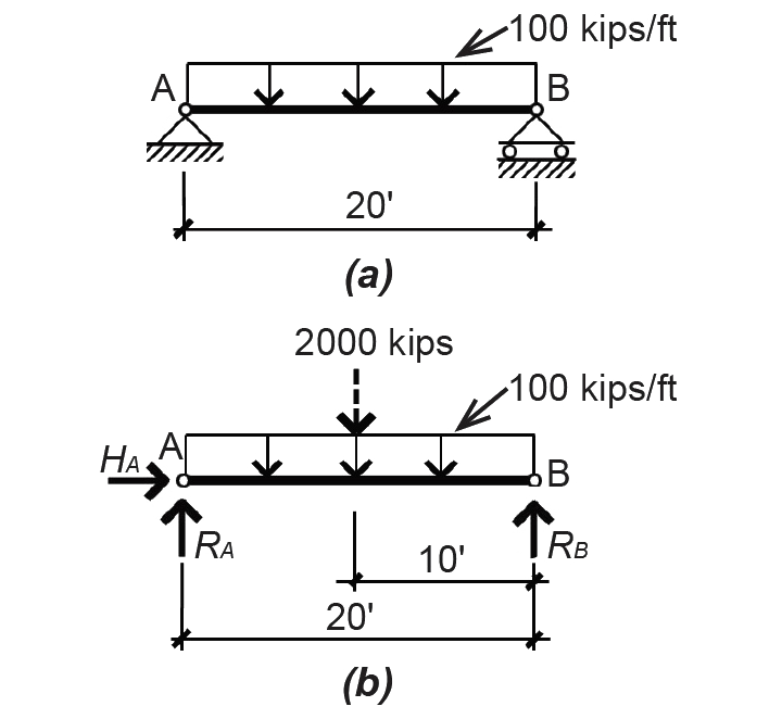
2. The solution to the horizontal reaction at point A is trivial, since no horizontal loads are present: ΣFx = HA = 0. In this equation, we use a sign convention, where positive corresponds to forces pointing to the right and negative to forces pointing to the left.
3. The order in which the remaining equations are solved is important: moment equilibrium is considered before vertical equilibrium in order to reduce the number of unknown variables in the vertical equilibrium equation. Moments can be taken about any point in the plane; however, unless you wish to solve the two remaining equations simultaneously, it is suggested that the point be chosen strategically to eliminate all but one of the unknown variables. Each moment is the product of a force times a distance called the moment arm; this moment arm is measured from the point about which moments are taken to the "line of action" of the force and is measured perpendicular to the line of action of the force.
Where the moment arm equals zero, the moment being considered is also zero, and the force "drops out" of the equation. For this reason, it is most convenient to select a point about which to take moments that is aligned with the line of action of either of the two unknown vertical reactions so that one of those unknown forces drops out of the equation of equilibrium. The sign of each moment is based on an arbitrary sign convention, with positive used when the moment causes a clockwise rotation of the beam considered as a free-body diagram and negative when a counterclockwise rotation results (the opposite convention could be chosen as well). In the equation that follows, each product of two numbers represents a force times a distance so that, taken together, they represent the sum of all moments acting on the beam. Any force whose moment arm is zero is left out.
ΣMB = RA(20) – 2000(10) = 0
Solving for the vertical reaction at point A, we get: RA = 1000 kips.
4. Finally, we use the third equation of equilibrium to find the last unknown reaction. Another sign convention is necessary for vertical equilibrium equations: we arbitrarily choose positive to represent an upward-acting force and negative to represent a downward-acting force.
ΣFy = RA + RB – 2000 = 0
or, substituting RA = 1000 kips:
1000 + RB – 2000 = 0
Solving for the vertical reaction at point B, we get RB = 1000 kips. The two vertical reactions in this example are equal and could have been found by simply dividing the total load in half, as we did when considering tributary areas. Doing this, however, is only appropriate when the structure's geometry and loads are symmetrical.
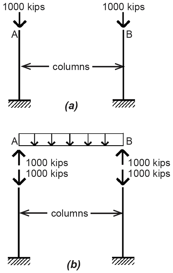
If the reactions represent other structural supports such as columns or girders, then the "upward" support they give to the beam occurs simultaneously with the beam's "downward" weight on the supports: in other words, if the beam in Example 1.1 is supported on two columns, then those columns (at points A and B) would have load diagrams as shown in Figure 1.16a. The beam and columns, shown together, have reactions and loads as shown in Figure 1.16b. These pairs of equal and opposite forces are actually inseparable. In the Newtonian framework, each action, or load, has an equal reaction.
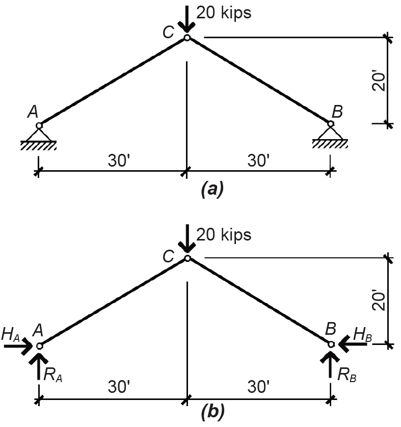
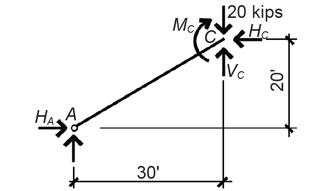
Problem definition. Find the reactions for the three-hinged arch shown in Figure 1.17a.
Solution overview. Draw load diagram with unknown forces and/or moments replacing the reaction (constraint) symbols; use the three equations of equilibrium, plus one additional equation found by considering the equilibrium of another free-body diagram, to find the four unknown reactions.
Problem solution
1. The three-hinged arch shown in this example appears to have too many unknown variables (four unknowns versus only three equations of equilibrium); however, the internal hinge at point C prevents the structure from behaving as a rigid body, and a fourth equation can be developed out of this condition. The initial three equations of equilibrium can be written as follows: a. ΣMB = RA(60) – 20(30) = 0, from which RA = 10 kips. b. ΣFy = RA + RB – 20 = 0; then, substituting RA = 10 kips from the moment equilibrium equation solved in step a, we get 10 + RB – 20 = 0, from which RB = 10 kips. c. ΣFx = HA – HB = 0.
Sign conventions are as described in Example 1.1. This last equation of horizontal equilibrium (step c) contains two unknown variables and cannot be solved at this point. To find HA, it is necessary to first cut a new FBD at the internal hinge (point C) in order to examine the equilibrium of the resulting partial structure shown in Figure 1.18.
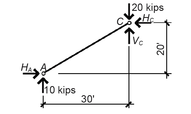
2. With respect to this FBD, we show unknown internal forces HC and VC at the cut, but we show no bending moment at that point since none can exist at a hinge. This condition of zero moment is what allows us to write an equation that can be solved for the unknown, HA:
ΣMC = 10(30) – HA(20) = 0
from which HA = 15 kips.
Then, going back to the "horizontal" equilibrium equation shown in step c that was written for the entire structure (not just the cut FBD), we get:
ΣFx = HA – HB = 15 – HB = 0
from which HB = 15 kips.
While the moment equation written for the FBD can be taken about any point in the plane of the structure, it is easier to take moments about point C, so that only HA appears in the equation as an unknown. Otherwise, it would be necessary to first solve for the internal unknown forces at point C, using "vertical" and "horizontal" equilibrium.
If there were no hinge at point C, we would need to add an unknown internal moment at C, in addition to the forces shown (Figure 1.19). The moment equation would then be ΣMC = 10(30) – HA(20) + MC = 0. With two unknown variables in the equation (HA and MC), we cannot solve for HA. In other words, unlike the three-hinged arch, this two-hinged arch is an indeterminate structure.
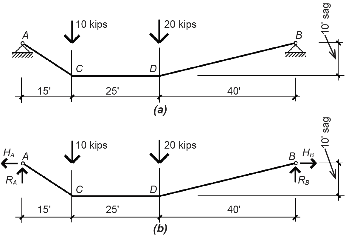
Problem definition. Find the reactions for the flexible cable structure shown in Figure 1.20a. The actual shape of the cable is unknown: all that is specified is the maximum distance of the cable below the level of the supports (reactions): the cable's sag.
Solution overview. Draw load diagram with unknown forces and/or moments replacing the reaction (constraint) symbols; use the three equations of equilibrium, plus one additional equation found by considering the equilibrium of another free-body diagram, to find the four unknown reactions.
Problem solution
1. The cable shown in this example appears to have too many unknown variables (four unknowns versus only three equations of equilibrium); however, the cable's flexibility prevents it from behaving as a rigid body, and a fourth equation can be developed out of this condition. The three equations of equilibrium can be written as follows:
a. ΣMB = RA(80) – 10(65) – 20(40) = 0, from which RA = 18.125 kips.
b. ΣFy = RA + RB – 10 – 20 = 0; then, substituting RA = 18.125 kips from the moment equilibrium equation solved in step a, we get 18.125 + RB – 10 – 20 = 0, from which RB = 11.875 kips.
c. ΣFx = –HA + HB = 0.
Sign conventions are as described in Example 1.1. This last equation of horizontal equilibrium (step c) contains two unknown variables and cannot be solved at this point. By analogy to the three-hinged arch, we would expect to cut an FBD and develop a fourth equation. Like the internal hinge in the arch, the entire cable, being flexible, is incapable of resisting any bending moments. But unlike the arch, the cable's geometry is not predetermined; it is conditioned by the particular loads placed upon it. Before cutting the FBD, we need to figure out where the maximum specified sag of 10 ft occurs: without this information, we would be writing a moment equilibrium equation of an FBD in which the moment arm of the horizontal reaction, HA, was unknown.
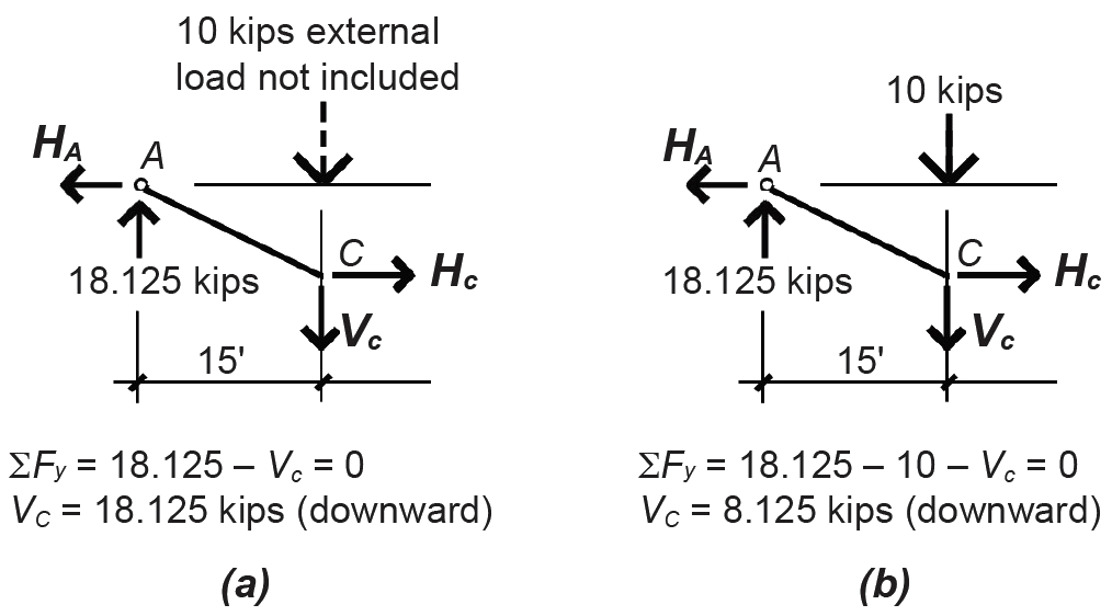
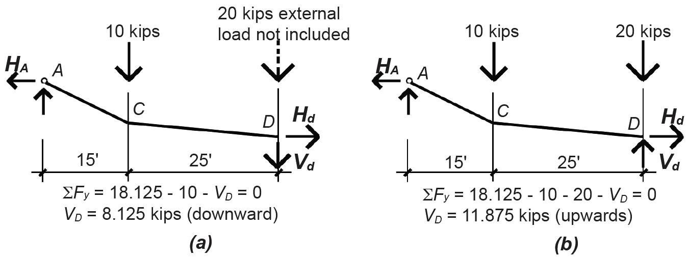
2. We find the location of the sag point by looking at internal vertical forces within the cable. When the direction of these internal vertical forces changes, the cable has reached its lowest point (Figure 1.21). Checking first at point C, we see that the internal vertical force does not change direction on either side of the external load of 10 kips (comparing Figure 1.22a and Figure 1.22b), so the sag point cannot be at point C.
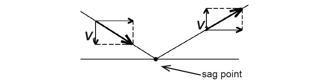
However, when we check point D, we see that the direction of the internal vertical force does change, as shown in Figure 1.23. Thus, point D is the sag point of the cable (i.e., the low point), specified as being 10 ft below the support elevation.
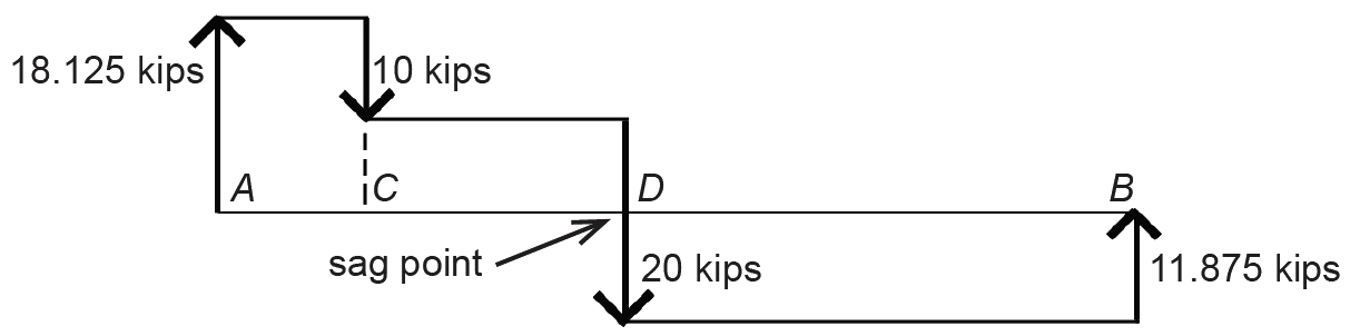
We can also find this sag point by constructing a diagram of cumulative vertical loads, beginning on the left side of the cable (Figure 1.24). The sag point then occurs where the "cumulative force line" crosses the baseline.
3. Having determined the sag point, we cut an FBD at that point (Figure 1.25a) and proceed as in the example of the three-hinged arch, taking moments about the sag point: ΣMD = 18.125(40) – 10(25) – 10(HA) = 0, from which HA = 47.5 kips.
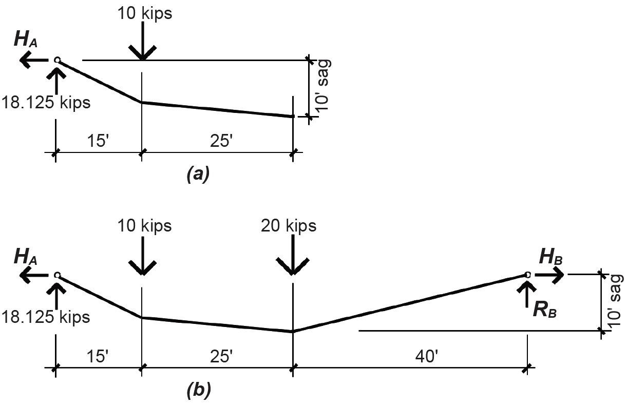
Once the location of the sag point is known, a more accurate sketch of the cable shape can be made, as shown in Figure 1.25b.
Then, going back to the "horizontal" equilibrium equation shown in step 1c that was written for the entire structure (not just the cut FBD), we get ΣFx = –HA + HB = –47.5 + HB = 0, from which HB = 47.5 kips. In this last equation, the value of HA is written with a minus sign since it acts toward the left (and our sign convention has positive going to the right).
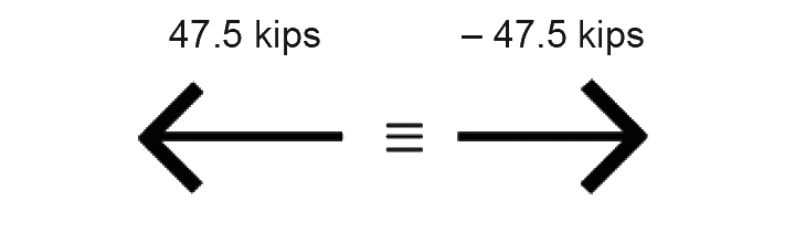
We have thus far assumed particular directions for our unknown forces — for example, that HA acts toward the left. Doing so resulted in a positive answer of 47.5 kips, which confirmed that our guess of the force's direction was correct. Had we initially assumed that HA acted toward the right, we would have gotten an answer of –47.5 kips, which is equally correct, but less satisfying. In other words, both ways of describing the force shown in Figure 1.26 are equivalent.
© 2020 Jonathan Ochshorn; all rights reserved. This section first posted November 15, 2020; last updated November 15, 2020.