
Contents |
Introduction to structural design | Statics | Tributary areas | Equilibrium | Reactions |
Finding internal forces and moments is no different than finding reactions; one need only cut an FBD at the cross section where the internal forces and moments are to be computed (after having found any unknown reactions that occur within the diagram). At any cut in a rigid element of a plane structure, two perpendicular forces and one moment are potentially present. These internal forces and moments have names, depending on their orientation relative to the axis of the structural element where the cut is made (Figure 1.27). The force parallel to the axis of the member is called an axial force; the force perpendicular to the member is called a shear force; the moment about an axis perpendicular to the structure's plane is called a bending moment.
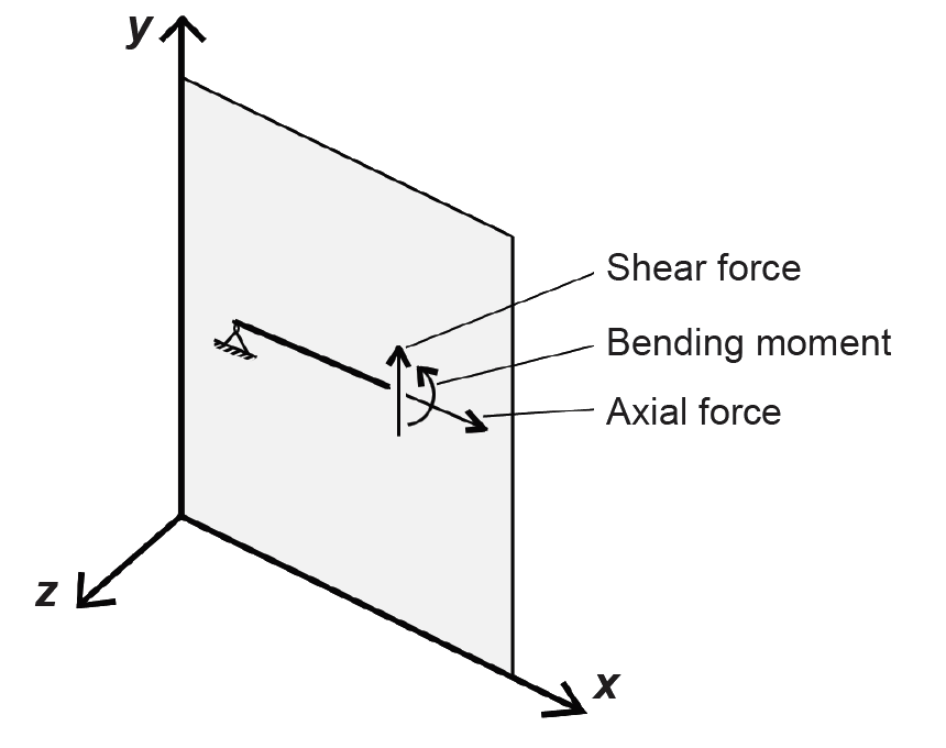
In a three-dimensional environment with x-, y-, and z-axes as shown in Figure 1.27, three additional forces and moments may be present: another shear force (along the z-axis) and two other moments, one about the y-axis and one about the x-axis. Moments about the y-axis cause bending (but bending perpendicular to the two-dimensional plane); moments about the x-axis cause twisting or torsion. These types of three-dimensional structural behaviors are beyond the scope of this discussion.
Where the only external forces acting on beams are perpendicular to a simply supported beam's longitudinal axis, no axial forces can be present. The following examples show how internal shear forces and bending moments can be computed along the length of the beam.
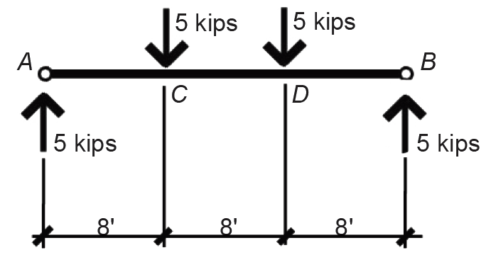
Problem definition. Find internal shear forces and bending moments at key points along the length of the beam shown in Figure 1.28, i.e., under each external load and reaction. Reactions have already been determined.
Solution overview. Cut free-body diagrams at each external load; use equations of equilibrium to compute the unknown internal forces and moments at those cut points.
Problem solution
1. To find the internal shear force and bending moment at point A, first cut a free-body diagram there, as shown in Figure 1.29. Using the equation of vertical equilibrium, ΣFy = 5 – VA = 0, from which the internal shear force VA = 5 kips (downward). Moment equilibrium is used to confirm that the internal moment at the hinge is zero: ΣMA = MA = 0. The two forces present (5 kips and VA = 5 kips) do not need to be included in this equation of moment equilibrium since their moment arms are equal to zero. The potential internal moment, MA, is entered into the moment equilibrium equation as it is (without being multiplied by a moment arm) since it is already, by definition, a moment.

2. Shear forces must be computed on "both sides" of the external load at point C; the fact that this results in two different values for shear at this point is not a paradox: it simply reflects the discontinuity in the value of shear caused by the presence of a concentrated load. In fact, a truly concentrated load acting over an area of zero is impossible, since it would result in an infinitely high stress at the point of application; all concentrated loads are really distributed loads over small areas. However, there is only one value for bending moment at point C, whether or not the external load is included in the FBD. In other words, unlike shear force, there is no discontinuity in moment resulting from a concentrated load.
a. Find internal shear force and bending moment at point C, just to the left of the external load, by cutting an FBD at that point as shown in Figure 1.30a. Using the equation of vertical equilibrium: ΣFy = 5 – VC = 0, from which the internal shear force VC = 5 kips (downward). Using the equation of moment equilibrium, ΣMC = 5(8) – MC = 0, from which MC = 40 ft-kips (counterclockwise).
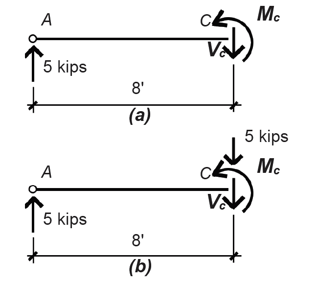
b. Find internal shear force and bending moment at point C, just to the right of the external load by cutting a FBD at that point, as shown in Figure 1.30b. Using the equation of vertical equilibrium: ΣFy = 5 – 5 – VC = 0, from which the internal shear force VC = 0 kips. Using the equation of moment equilibrium, ΣMC = 5(8) – MC = 0, from which MC = 40 ft-kips (counterclockwise), as before.
3. Find shear and moment at point D.
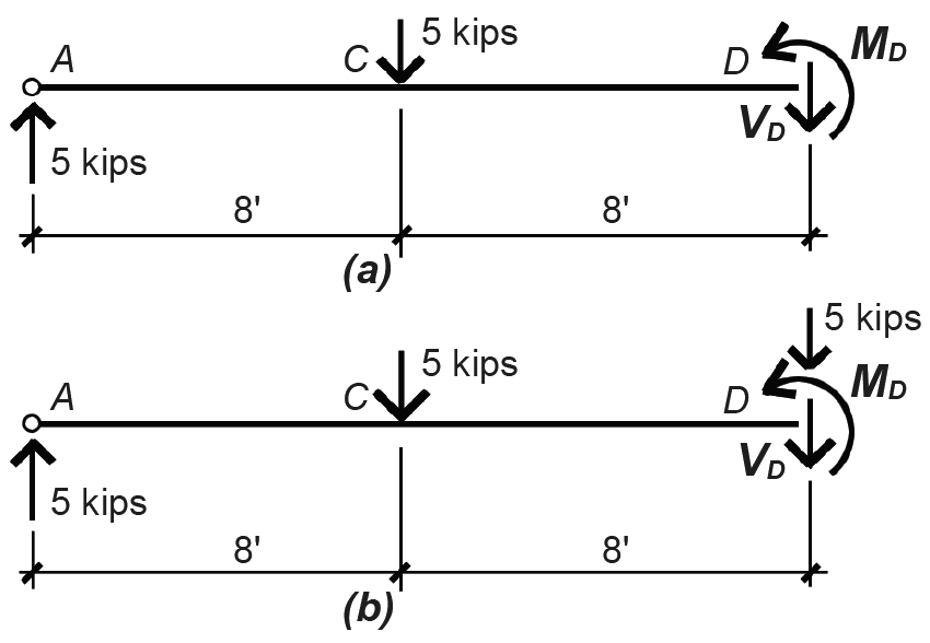
a. Find internal shear force and bending moment at point D, just to the left of the external load by cutting an FBD at that point, as shown in Figure 1.31a. Using the equation of vertical equilibrium: ΣFy = 5 – 5 – VD = 0, from which the internal shear force VD = 0 kips. Using the equation of moment equilibrium, ΣMD = 5(16) – 5(8) – MD = 0, from which MD = 40 ft-kips (counterclockwise).
b. Find internal shear force and bending moment at point D, just to the right of the external load by cutting an FBD at that point, as shown in Figure 1.31b. Using the equation of vertical equilibrium, ΣFy = 5 – 5 – 5 – VD = 0, from which the internal shear force VD = –5 kips (downward), which is equivalent to 5 kips (upward). Using the equation of moment equilibrium, ΣMD = 5(16) – 5(8) – MD = 0, from which MD = 40 ft-kips (counterclockwise), as before.
4. Find shear and moment at point B by cutting a free-body diagram just to the left of the reaction at point B, as shown in Figure 1.32. Using the equation of vertical equilibrium, ΣFy = 5 – 5 – 5 – VB = 0, from which the internal shear force VB = –5 kips (downward), which is equivalent to 5 kips (upward).
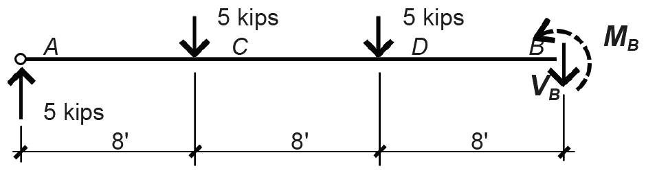
Moment equilibrium is used to confirm that the internal moment at the hinge is zero: ΣMB = 5(24) – 5(16) – 5(8) – MB = 0, from which MB = 0. The internal shear force, VB, does not need to be included in this equation of moment equilibrium since its moment arm is equal to zero. The forces and moments can be graphically displayed as shown in Figure 1.33, by connecting the points found earlier.
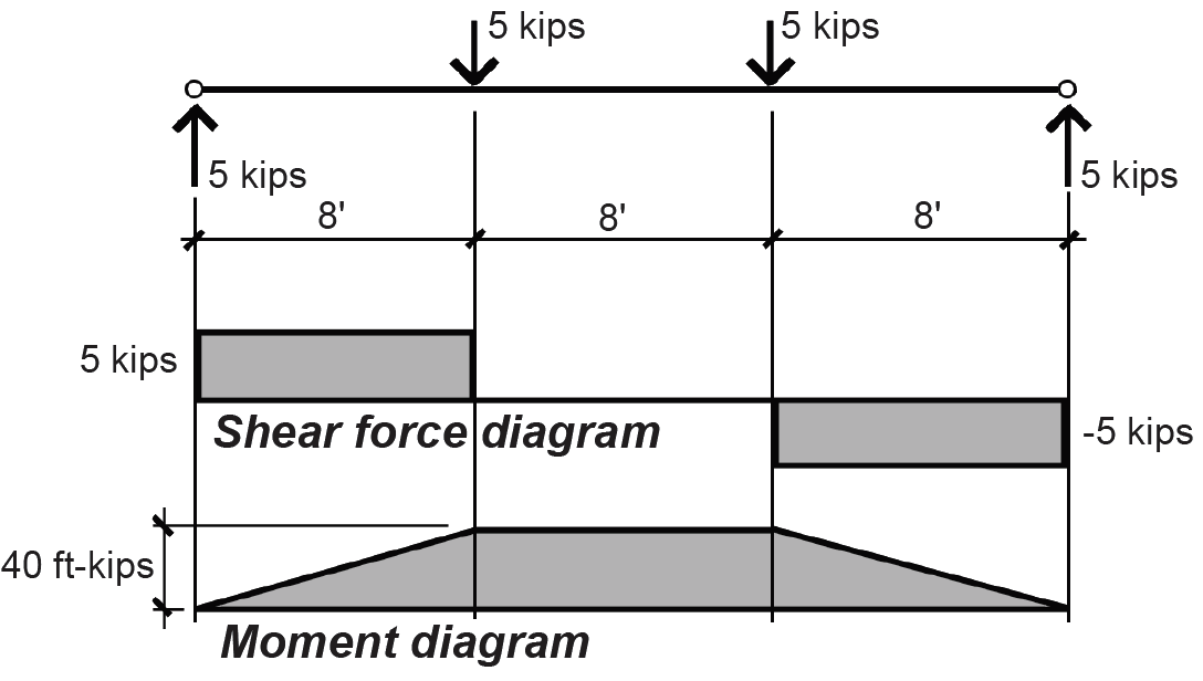
Some important characteristics of internal shear forces and bending moments may now be summarized: (1) Internal axial forces are always zero in a horizontally oriented simply supported beam with only vertical loads. (2) Moments at hinges at the ends of structural members are zero. Only when a continuous member passes over a hinge can the moment at a hinge be nonzero. (3) A shear force acting downward on the right side of an FBD is arbitrarily called "positive"; a bending moment acting counterclockwise on the right side of an FBD is arbitrarily called "positive." Positive bending corresponds to "tension" on the bottom and "compression" on the top of a horizontal structural element.
Shear and moment diagrams can also be drawn by noting the following rules: (1) At any point along the beam, the slope of the shear diagram equals the value of the load (the "infinite" slope of the shear diagram at concentrated loads can be seen as a shorthand approximation to the actual condition of the load being distributed over some finite length, rather than existing at a point). (2) Between any two points along a beam, the change in the value of shear equals the total load (between those points). (3) The slope of the moment diagram at any point equals the value of the shear force at that point. (4) The change in the value of bending moment between any two points equals the "area of the shear diagram" between those points. These rules are derived by applying the equations of equilibrium to an elemental slice of a beam, as shown in Appendix Table A-1.1.
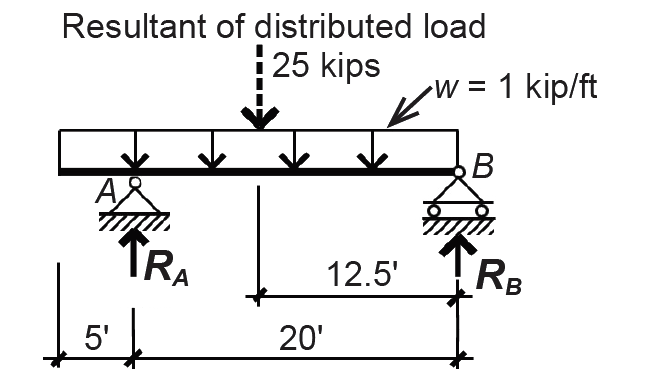
Problem definition. Find the distribution of internal shear forces and bending moments for the beam shown in Figure 1.34, first by using FBDs and then by applying the rules from Appendix Table A-1.1.
Solution overview. Find reactions using the equations of equilibrium; find internal shear force and bending moment at key points (at reactions and at location of zero shear).
Problem solution
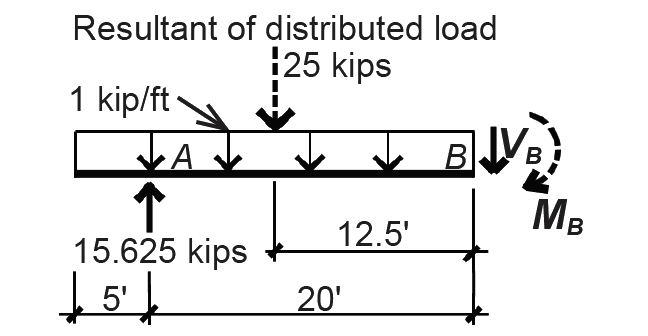
1. Find the resultant of the distributed load, equal to 1 kip/ft × 25 ft = 25 kips.
2. To find reactions, first take moments about either point A or point B; we choose point B: ΣMB = RA(20) – 25(12.5) = 0, from which RA = 15.625 kips. Next, use the equation of vertical equilibrium to find the other reaction: ΣFy = RA + RB – 25 = 15.625 + RB – 25 = 0, from which RB = 9.375 kips.
3. Find shear and moment at point A.
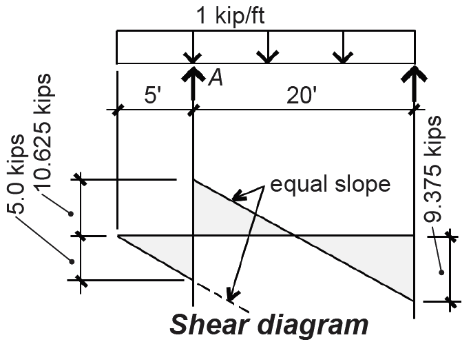
a. Find internal shear force and bending moment at point A, just to the left of the reaction by cutting an FBD at that point, as shown in Figure 1.35a. Using the equation of vertical equilibrium, ΣFy = –5 – VA = 0, from which the internal shear force, VA = –5 kips (downward) or 5 kips (upward). Using the equation of moment equilibrium, ΣMA = –5(2.5) – MA = 0, from which MA = –12.5 ft-kips (counterclockwise) or 12.5 ft-kips (clockwise).
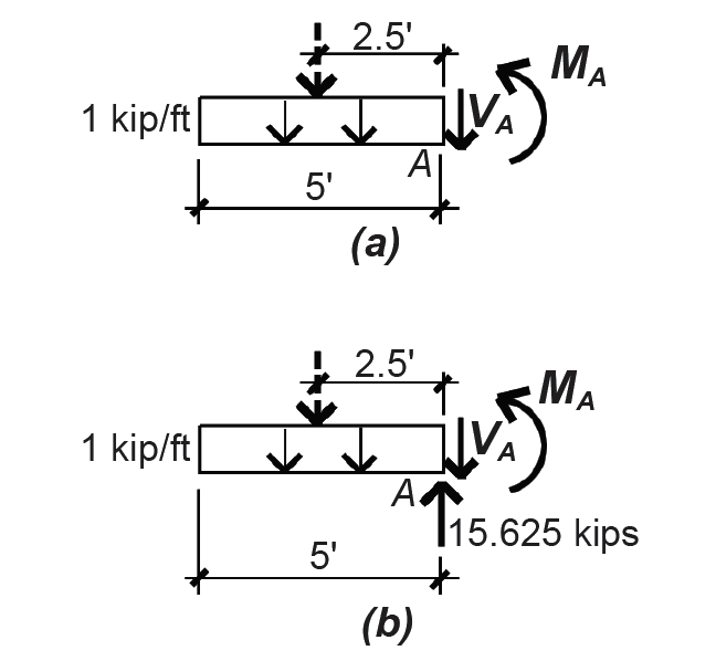
b. Find internal shear force and bending moment at point A, just to the right of the reaction by cutting an FBD at that point, as shown in Figure 1.35b. Using the equation of vertical equilibrium, ΣFy = 15.625 – 5 – VA = 0, from which the internal shear force VA = 10.625 kips (downward). Using the equation of moment equilibrium, ΣMA = –5(2.5) – MA = 0, from which MA = –12.5 ft-kips (counterclockwise) or 12.5 ft-kips (clockwise), as before.
The moment at point A is not zero, even though there is a hinge at that point. The reason is that the beam itself is continuous over the hinge. This continuity is essential for the stability of the cantilevered portion of the beam.
4. Find shear and moment at point B by cutting a free-body diagram just to the left of the reaction at point B, as shown in Figure 1.36. Using the equation of vertical equilibrium, ΣFy = 15.625 – 25 – VB = 0, from which the internal shear force VB = – 9.375 kips (downward), which is equivalent to 9.375 kips (upward). Moment equilibrium is used to confirm that the internal moment at the hinge is zero: ΣMB = 15.625(20) – 25(12.5) + MB = 0, from which MB = 0. The internal shear force, VB, does not need to be included in this equation of moment equilibrium since its moment arm is equal to zero.
5. The internal shear forces can be graphically displayed as shown in Figure 1.37, by connecting the points found earlier. The slope of the shear diagram at any point equals the value of the load; since the load is uniformly distributed, or constant, the slope of the shear diagram is also constant.
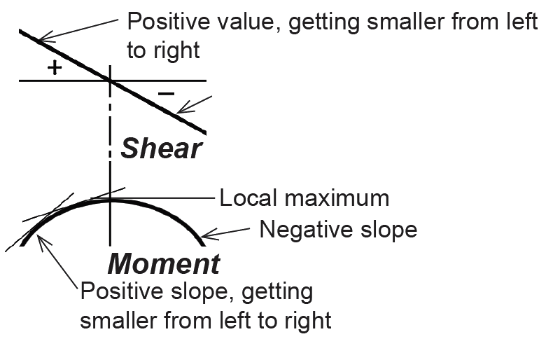
The bending moment cannot be adequately diagrammed until one more point is determined and analyzed: the point somewhere between the two reactions where the shear is zero. Since the slope of the moment diagram at any point equals the value of the shear force, a change from positive to negative shear indicates at least a "local" minimum or maximum moment (Figure 1.38).
This key point, labeled C in Figure 1.39, can be located by dividing the value of shear just to the right of the reaction at point A by the distributed load: the distance of point C from point A, then, is x = 10.625/1.0 = 10.625 ft.
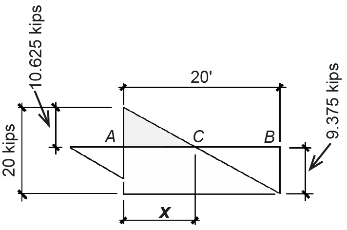
The length, x, can also be found using similar triangles: x/10.625 = 20/20. Solving for x, we get the same value as earlier: x = 10.625 ft.
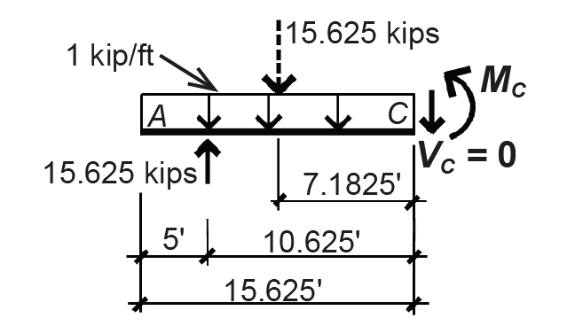
The moment at this point can be found by cutting an FBD at point C, as shown in Figure 1.40, and applying the equation of moment equilibrium: ΣMC = 15.625(10.625) – 15.625(7.8125) – MC = 0, from which MC = 43.9 ft-kips (counterclockwise).
6. Alternatively, shear and moment diagrams may be drawn based on the rules listed in Appendix Table A-1.1, and illustrated in Figure 1.41. The critical points of the shear diagram are derived from the load diagram based on Rule 2: the "areas" of the load diagram (with concentrated loads or reactions counting as areas b and d) between any two points equal the change in shear between those points. These "area" values are summarized in the box between the load and shear diagrams. Connecting the points established using Rule 2 is facilitated by reference to Rule 1: the slope of the shear diagram equals the value of the load at that point. Therefore, where the load diagram is "flat" (i.e., has constant value), the shear diagram has constant slope represented by a straight line that has positive slope for positive values of load, and negative slope corresponding to negative values of load. Since almost all distributed loads are downward-acting (negative value), shear diagrams often have the characteristic pattern of negative slope shown in Figure 1.41.
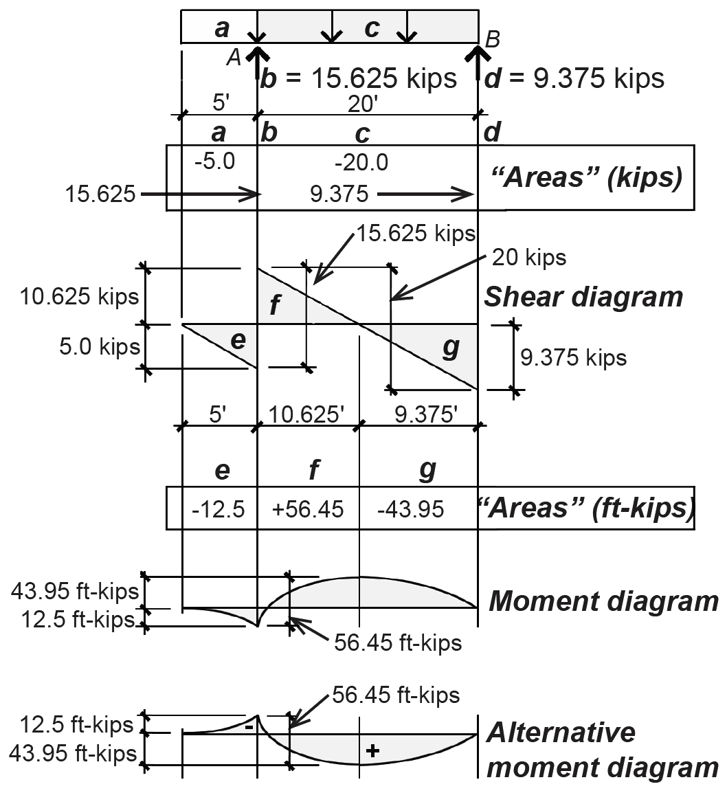
Once the shear diagram has been completed, and any critical lengths have been found (see step 5), the moment diagram can be drawn based on Rules 3 and 4 of Appendix Table A-1.1. Critical moments are first found by examining the "areas" under the shear diagram, as described in Rule 4 of Appendix Table A-1.1. These "areas" — actually forces times distances, or moments — are shown in the box between the shear and moment diagrams in Figure 1.41 and represent the change in moment between the two points bracketed by the shear diagram areas — not the value of the moments themselves. For example, the first "area e" of –12.5 ft-kips is added to the initial moment of zero at the free end of the cantilever, so that the actual moment at point A is 0 + –12.5 = –12.5 ft-kips. The maximum moment (where the shear is zero), is found by adding "area f " to the moment at point A: 56.45 + –12.5 = 43.95 ft-kips, as shown in Figure 1.41. Finally, slopes of the moment diagram curve can be determined based on Rule 3 of Appendix Table A-1.1: the slope of the moment diagram is equal to the value of the shear force at any point, as illustrated in Figure 1.38. moment (Figure 1.38).
In drawing the moment diagram, it is important to emphasize the following: (1) The area under the shear diagram between any two points corresponds, not to the value of the moment, but to the change in moment between those two points. Therefore, the triangular shear diagram area, f, of 56.45 ft-kips in the Example 1.5 does not show up as a moment anywhere in the beam; in fact, the maximum moment turns out to be 43.95 ft-kips. (2) The particular curvature of the moment diagram can be found by relating the slope of the curve to the changing values of the shear diagram. (3) The moment and shear diagrams are created with respect to the actual distribution of loads on the beam, not the resultants of those loads, which may have been used in the calculation of reactions. The location of the maximum moment, therefore, has nothing to do with the location of any resultant load but occurs at the point of zero shear. (4) Moment diagrams can also be drawn in an alternate form, as shown at the bottom of Figure 1.41, by reversing the positions of negative and positive values. This form has the benefit of aligning the shape of the moment diagram more closely with the deflected shape of the beam (although it still remains significantly different from the deflected shape), at the expense of being mathematically inconsistent. (5) Finally, it may be important in some cases to account for both positive and negative moments, and not just the maximum moment. In this example, the maximum positive moment is 43.95 ft-kips, while the maximum negative moment is 12.5 ft-kips.
There is a class of determinate structures that cannot sustain internal shear forces or bending moments, either because their component elements are pinned together or because they are inherently flexible. We will examine three types of these axial-force structures. Trusses are made from individual elements organized in a triangular pattern and assumed to be pinned at the joints so that they may be analyzed using only equations of equilibrium. Reactions of trusses are found just like the reactions of beams, while the reactions of three-hinged arches and cables — the other two axial-force structures already examined — require special treatment. In general, the axial forces within trusses, three-hinged arches, and cables are found using the three equations of equilibrium. The following examples illustrate specific techniques and strategies.
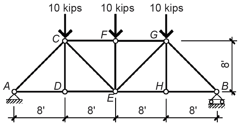
Problem definition. Find the internal axial forces in truss bars C-F, C-E, and D-E for the truss shown in Figure 1.42. Assume pinned joints, as shown.
Solution overview. Find reactions; then, using the so-called section method, cut a free-body diagram through the bars for which internal forces are being computed. As there are only three equations of equilibrium, no more than three bars may be cut (resulting in three unknown forces); use equations of equilibrium to solve for the unknown forces.
Problem solution
1. Find reactions: by symmetry, RA = RB = (10 + 10 + 10)/2 = 15 kips. Alternatively, one could take moments about point A or B, solve for the unknown reaction, and then use the equation of vertical equilibrium to find the other unknown reaction.
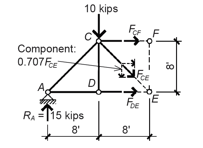
2. Cut a free-body diagram through the bars being evaluated (cutting through no more than three bars) as shown in Figure 1.43. Bar forces are labeled according to the nodes that are at either end of their bars, so, for example, FCF is the force between nodes C and F.
a. Show unknown axial forces as tension forces; a negative result indicates that the bar is actually in compression. Tension means that the force is shown "pulling" on the bar or node within the free-body diagram.
b. Use equilibrium equations, chosen strategically, to solve for unknown bar forces. To find FCF: ΣME = 15(16) – 10(8) + FCF(8) = 0; solving for the unknown bar force, we get FCF = –20 k (compression).
c. To find FDE: ΣMC = 15(8) – FDE(8) = 0; solving for the unknown bar force, we get FDE = 15k (tension).
d. Finally, to find FCE: find force "components" of inclined internal axial force FCE. The components can be found using principles of trigonometry, based on the geometry of the triangle determined by the 8 ft × 8 ft truss panels. For example, the vertical (or horizontal) component equals FCE × sin 45° = 0.707FCE. We then use the equation of vertical equilibrium: ΣFy = 15 – 10 – 0.707FCE = 0; solving for the unknown bar force, we get FCE = 7.07 kips (tension).
The assumption that only axial forces exist within a truss is valid when the following conditions are met: (1) all bar joints are "pinned" (hinged), and (2) external loads and reactions are placed only at the joints or nodes. Under these circumstances, no internal shear forces or bending moments are possible. In practice, modern trusses are rarely pinned at each joint; nevertheless, the assumption is often used for preliminary design since it facilitates the calculation of internal forces. What is more, actual bar forces in indeterminate trusses (i.e., where the members are continuous rather than pinned) are often reasonably close to the approximate results obtained by assuming pinned joints.
Problem definition. Find the internal axial force in bar AC of the three-hinged arch analyzed in Example 1.2.
Solution overview. Cut a free-body diagram through the bar in question, as shown in Figure 1.44a; label the unknown bar force as if in tension; use the equations of equilibrium to solve for the unknown force.
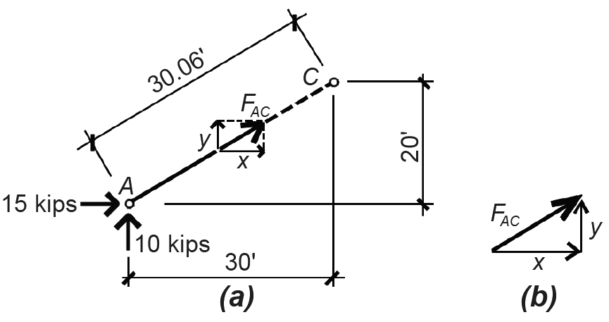
Problem solution
1. Because the far force, FAC, is inclined, it is convenient to draw and label its horizontal and vertical component forces, x and y. Using the equations of vertical and horizontal equilibrium, we can find these component forces directly: ΣFy = 10 + y = 0, from which y = –10 kips; ΣFx = 15 + x = 0, from which x = –15 kips. In both cases, the negative sign indicates that our initial assumption of tension was incorrect; the bar force is actually in compression, as one would expect in such an arch.
2. To find the actual bar force, FAC, the most direct approach is to use the Pythagorean theorem, with the unknown force being the hypotenuse of a right triangle, as shown in Figure 1.44b. Therefore, FAC = ![]() =
= 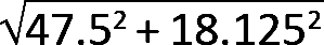 + 102 = 8.03 kips. The signs of the forces are omitted in this calculation.
Problem definition. Find the internal axial force in segment AC of the cable analyzed in Example 1.3.
Solution overview. Cut a free-body diagram through the segment in question, as shown in Figure 1.45; label unknown cable force as if in tension; use the equations of equilibrium to solve for the unknown force.
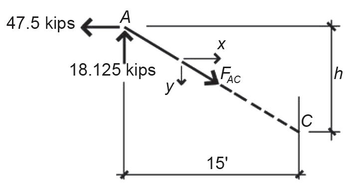
Problem solution
1. Because the cable force, FAC, is inclined, it is convenient to draw and label its horizontal and vertical component forces, x and y. Using the equations of vertical and horizontal equilibrium, we can find these component forces directly: ΣFy = 18.125 – y = 0, from which y = 18.125 kips; ΣFx = –47.5 + x = 0, from which x = 47.5 kips. In both cases, the positive sign indicates that our initial assumption of tension was correct, as one would expect in any cable structure.
2. To find the actual cable force, FAC, the most direct approach is to use the Pythagorean theorem, with the unknown force being the hypotenuse of a right triangle. Therefore, FAC = ![]() =
= 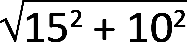 = 50.84 kips. The signs of the forces are omitted in this calculation.
3. Since the cable is flexible, the height,
© 2020 Jonathan Ochshorn; all rights reserved. This section first posted November 15, 2020; last updated November 15, 2020.